Introduction to Auto ML Time Series

What Is a Time Series?

A time series is a collection of data points recorded at regular time intervals — like daily sales, hourly temperature, or monthly website traffic. The main goal is to predict future values based on past patterns.

Example: You have a file that shows how many T-shirts were sold each day. You want to forecast sales for the next 7 days — that's a time series problem.

What Are We Predicting?

In a time series, we focus on one main thing to predict — this is called the target.

Target = the value we want to forecast.
Example: number of sales per day.

Timestamp = the date/time associated with each value.
Example: “2025-07-10”.

So each row in your data typically has:

timestamp   |   target
------------|-----------
2025-07-01  |     100
2025-07-02  |     120
...         |     ...

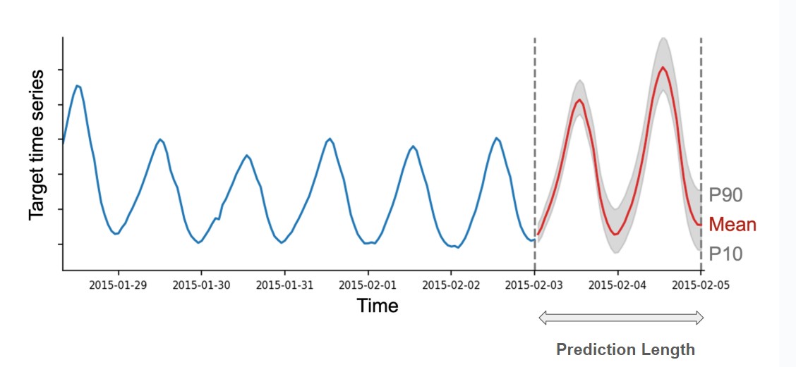
The prediction will be performed over a prediction length. This is the number of timestamps predicted in the future immediately after the last timestamp of the data.

The model learns patterns from past data of the target — so it's important to have enough historical data. Ideally:
At least 30–60 data points per series
More is better, especially for weekly or seasonal patterns

The variables that need to be supplied in a table:

⌛ Timestamps
Timestamps tell the model when each data point happened. They should be in a consistent format and evenly spaced (like daily, hourly, or monthly).
🎯 Target
The main value you want to predict — like sales, temperature, or revenue.
📈 Covariates (Optional)
Covariates are extra columns that might help with prediction. They can be:
- Known in advance (called "known covariates")
  Example: holiday dates, marketing campaigns, day of week
- Observed in the past only (called "past covariates")
  Example: number of site visits, temperature
These add context to your model and can improve predictions.

AutoML Timeseries can estimate ranges of likely values, not just one guess. These are called quantile forecasts. For example, if the 0.1 quantile (also known as P10, or the 10th percentile) is equal to x, it means that the time series value is predicted to be below x 10% of the target. As another example, the 0.5 quantile (P50) corresponds to the median forecast. Quantiles can be used to reason about the range of possible outcomes. For instance, by the definition of the quantiles, the time series is predicted to be between the P10 and P90 values with 80% probability.

Example:

10th percentile: a “low guess” (pessimistic)
50th percentile: the “most likely” guess (median)
90th percentile: a “high guess” (optimistic)

This helps with uncertainty — you can plan for best/worst-case scenarios.

What Models to use?

Different models are available for prediction. They are organized by types:

🧪 Baselines (Naive, Seasonal Naive, Average, Seasonal Average)
Simple models that repeat the last or seasonal values.

Best for: Benchmarks, debugging, simple data

✔️ Use when:
- You want to test whether other models are actually learning anything
- Your time series is highly regular (e.g., same value every day)
🔁 Statistical Models (ETS, AutoARIMA, AutoETS, AutoCES, Theta, NPTS)
These models are based on traditional time series techniques.

Best for: Small datasets, predictable trends or seasonality

Advantages:
- Fast training
- Easy to interpret
Use cases:
- Sales over time with clear seasonal trends
- Short-term predictions with few external variables
✔️ Use when:
- You need a fast, simple model
- You don’t have covariates (extra columns like holidays, promo, etc.)
Some statistical models (ADIDA, Croston, IMAPA) are built specifically for sparse and nonnegative data, especially for use in intermittent demand forecasting.
🧠 Deep Learning Models (DeepAR, TemporalFusionTransformer, TiDE, WaveNet)
These models use neural networks and can learn complex relationships.

Best for: Large datasets, multivariate time series, rich features

Advantages:
- Can incorporate many covariates
- Handle missing data and nonlinear patterns well
- Produce probabilistic forecasts (with quantiles)
Use cases:
- Forecasting demand across 1000+ SKUs
- Data with promotions, pricing, weather, holidays
- Long-range forecasting (weeks/months ahead)
✔️ Use when:
- You have lots of data
- You have multiple time series
- You want to include covariates
- You need uncertainty estimates (e.g., low/medium/high forecast bands)
🧮Tabular Models ( RecursiveTabularModel, DirectTabularModel)
Some models like LightGBM, CatBoost, or RandomForest can be applied to time series by reshaping the time series into a tabular format (aka Statistical + Machine Learning Hybrid).

Advantages:
- Great for short-term forecasts
- Support both past and future covariates
- Work well on small-to-medium multivariate datasets
- Use powerful AutoGluon tabular ensembling under the hood
✅ Use when:
- You are familiar with tabular data formats
- You have good covariates (like day-of-week, holiday, weather)
- You want fast, customizable results
🧠 Pretrained model (Chronos)
It is a powerful and recent deep-learning-based model, designed for flexibility, accuracy, and fast training.

How good is the prediction?

Forecasting metrics help us measure how good our predictions are by comparing the forecasted values to the actual (true) values. Several metrics, each useful in different situations, are availble.

Mean Weighted Quantile Loss (WQL)
Scaled Quantile Loss (SQL)
Mean Absolute Error (MAE)
Mean Absolute Percentage Error (MAPE)
Mean Absolute Scaled Error (MASE)
Mean Squared Error (MSE)
Root Mean Squared Error (RMSE)
Root Mean Squared Logarithmic Error (RMSLE)

If you are not sure which evaluation metric to pick, here are three questions that can help you make the right choice for your use case.

Are you interested in a point forecast or a probabilistic forecast?

If your goal is to generate an accurate probabilistic forecast, you should use WQL or SQL metrics. These metrics are based on the quantile loss and measure the accuracy of the quantile forecasts.

Do you care more about accurately predicting time series with large values?

If the answer is “yes” (for example, if it’s important to more accurately predict sales of popular products), you should use scale-dependent metrics like WQL, MAE, RMSE, or WAPE. These metrics are also well-suited for dealing with sparse (intermittent) time series that have lots of zeros.

(Point forecast only) Do you want to estimate the mean or the median?

To estimate the median, you need to use metrics such as MAE, MASE or WAPE. If your goal is to predict the mean (expected value), you should use MSE, RMSE or RMSSE metrics.

Using the evaluation option

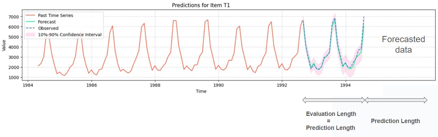
To help evaluate your model, you can use the evaluation option. With this option, AutoML will use the last datapoints of the historic data to evaluate the model more precisely, checking its prediction against the true data. The number of datapoints used for the evaluation is matching the prediction length. If the prediction length is 8 (timestamps), then the evaluation is performed on the last 8 rows of the selected historic data.

When using the evaluation option, the metric will be recalculated on the evaluation section and compared to historic value to estimate the best model.

Selection of data from tables

AutoML timeseries interface gives the option to select partial tables. By using the offset field it is possible to skip data from the beginning of the table. Also using data length allows to skip some data at the end of the table (especially if you want to estimate the model yourself with your own data). The prediction starts at the last selected rows.

You can have more than one timeserie in your table, either in row or columns. You will need to use ITEM_ID to separate the timeseries.